Posts

Showing posts from 2017

Row 1 Is Missing. How to unhide?
Image
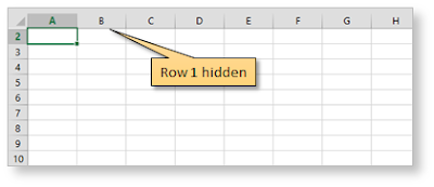
Excel Tip #030 Row 1 Is Missing. How to unhide? As you know, hiding and unhiding rows in Excel is simple as selecting them, right-clicking and choosing Hide or Unhide . The trick to selecting hidden rows, is to select a row above or below and then drag to included the hidden rows. For example, if you accidentally hide row 1 of your worksheet or inherit someone else's worksheet with one or more of the top rows hidden, you may be wondering how to unhide them since apparently you cannot select them. Row 1 Hidden There is a really easy solution. 1) Point to the row 2 header , press the left mouse button and drag upward to the top of the worksheet. Although you cannot see it, row 2 and row 1 are now selected 2) Right click anywhere on row 2 3) Choose Unhide from the right-click menu Unhiding hidden Row 1 NOTE : This also works for multiple hidden rows. There is another method of doing the same if Row 1 is hidden. 1) Go to the top left corner of the sheet abov...
Subtotal Dates By Month (or) Year

Image
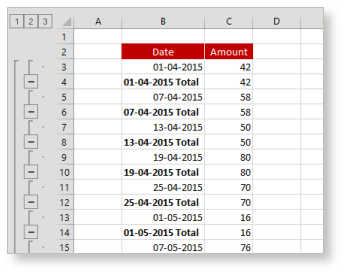
Excel Tip #029 Subtotal Dates By Month (or) Year There may be times when you want to subtotal your data by month and year, however simply Subtotaling a column of dates won't work because that will create a subtotal for each day. Subtotal Dates - Example Here's a trick you can use to create subtotals for each month while ignoring the day... 1) Sorted your dates by selecting a single date within the table and from the Data tab click the sort A>Z button; 2) Next you need to apply a date/number format that displays the month but not the day (e.g. mmm yyyy). To do this, from the Number group on the Home tab, click the Number Format dropdown (or press CTRL+1) and choose More Number Formats ..., then click Custom and enter mmm yyyy in the Type box. All of the dates now display the month and year (e.g. Apr 2015) Formatting Dates 3) To subtotal your data based on the month and year in the Date column, from the Data tab, click Subtotal,. in the Subtotal dial...

Use of Function keys in Excel

Image
Excel Tip #028 Use of Function keys in Excel Most of us know few function keys that are used as shortcuts in Excel, but hardly make use of it. Either because of the keyboard settings or due to the scarcity of the knowledge. Below, the use of function keys are tabulated along with their combinations which will make your life much more easier. Function Key = F1 to F8 Function Key = F9 to F12 Try to use these Function key shortcuts in your day to day tasks and be benefited.

Find And Replace Cell Colors

Excel Tip #027 Find And Replace Cell Colors It is common for Excel users to apply background colors to cells, such as green to indicate for positive, red to indicate warning etc. But how to remove the green fill color from hundreds of cells throughout the workbook without having to do them one by one. Steps to Find cells with a specific Fill color      1) Press CTRL+F to open the Find dialog       2) If you don't see the Format button, click the Options>> button       3) Click the Format... button       4) Click each of the tabs (Number, Alignment, Font, Border, Fill and Protection) and, if the Clear button isn't 'grayed out', click it to clear any formatting from the search criteria       5) Click the Fill tab and choose the color you wish to find     6) Click the Find All button. All of the cells with the Fill color you selected will be listed at the bottom of the Find an...

Move Columns & Rows Quickly

Image
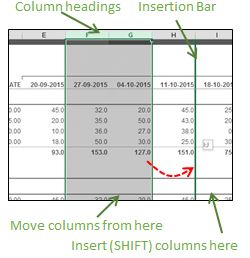
Excel Tip #026 Move Columns & Rows Quickly I often see Excel users 'moving' a column by inserting a blank column where they want to move the column, drag the original column and drop it in the empty column, the go back and delete the empty original column. Same thing for rows. There is a much, much easier and faster way! Move Columns To move a column (or multiple columns) and insert it (them) between two other columns,       1) Select the column(s) you want to move      2)   Hold down the SHIFT key. Holding down SHIFT tells Excel to 'insert' the columns      3)   Point to the edge of the selected column(s)      4)   Press and hold your left mouse button to drag and position the 'insertion bar' where you want to move the column(s)      5)   Release the mouse button, then release the SHIFT key Move Columns Alternatively,  Right-click column heading you w...

Return the last value in a list

Image
Excel Tip #025 Return the last value in a list You would have faced some situations where you want to get the last value in the list. And this list will not be static, the list will grow further and still the the last value has to be returned . Quite interesting...! There might be multiple ways but as far I know, there are 2 ways in which we can get this done. But as far I consider, there are loopholes in all the 2 methods . Let us get in detail with all the 2 methods. Method 1 This method uses the function LOOKUP . Let us see get to know about this function. LOOKUP function returns a value from a range (one row or one column) or from an array. The syntax is: LOOKUP( lookup_value, lookup_range, [result_range] ) (or) LOOKUP( lookup_value, lookup_range ) We are going to use a hidden excel function in this method which is 9e9 . So what does this 9e9 give?  9e9 is just a notation for 9,000,000,000 which is considered as the largest value in the array...

Calculate Weighted Average

Image
Excel Tip #024 Calculate Weighted Average Excel makes it extremely easy to calculate the average of data by using the AVERAGE function. But what if some of the values have more "weight" than others? For those cases, you'll need to calculate the Weighted Average . Although Excel doesn't have a weighted average function, it does have a function that does most of the work for you: SUMPRODUCT . In order to calculate the weighted average, we are having 2 columns of data. The first column contains the grades for each assignment and the second column contains the weights. A higher weight will cause the data (assignment) to have a greater effect on the final grade. The weights can also be greater than 100% but it would be meaningful if it is 100% Below is the example data containing 5 assignments along with their marks and the weights. Example - Weighted Average Before going to the example, let us learn about SUMPRODUCT. This function multiplies the correspo...

Prevent Automatic Hyperlinks in Excel

Image
Excel Tip #023 Prevent Automatic Hyperlinks Having Hyperlinks in your worksheet that allow you to quickly and easily open other related workbooks, can save you a lot of time. You don't have to browse to the folder where the workbook is located. Many of us use hyperlinks to jump from one sheet of the workbook to another sheet (or) to another workbook. But it can be annoying sometimes when you simply want to enter the data (e.g. website (or) email address) in your worksheet and it automatically gets created as hyperlinks. By clicking the Undo command (on the Quick Access Toolbar) or pressing CTRL+Z immediately after you create the hyperlink, you can quickly disable that hyperlink but that is not going to be a permanent solution. If you just don't want hyperlinks created in your workbooks every time you type a website (or) email address, you can disable this feature in Excel's options. From the File tab, click Options, Proofing , then click the AutoCorrect Opt...

Search Backwards in Excel

Excel Tip #022 Search Backwards in Excel Sometimes we take some things for granted in Excel and assume that everyone else knows too. Here's a tip which lot of Excel users don't know about it. Many Excel users know that the quickest way to find something in a large worksheet is to use Excel's Find command. On the Home tab, in the Editing group, click Find & Select , then Find or, preferrably, use the keyboard shortcut CTRL+F instead. Each time you click Find Next you will be taken to the next matching cell, starting from the active cell and going down the sheet until you finally come to the last one. But what if you want to find the 'last' matching value in a sheet and there are dozens or even hundreds of matching values? You don't want to click through each one until you finally reach the end. Here's a simple trick that will save you some time. Select a cell below the range you want to search ( CTRL+END is a shortcut you can use to quick...

Quickly Identify Column Differences

Image
Excel Tip #021 Quickly Identify Column Differences If you need to compare two or more columns of data, there are various methods you can use in Excel to check for differences. Sorting, Conditional Formatting and using formulas such as MATCH or VLOOKUP are just a few of them. For years, whenever I needed to compare two columns of data, I used a simple formula such as =B2=C2 that would give me TRUE if the cells are the same and FALSE if they aren't. But there's and even easier and faster way identify differences in columns of data without using formulas. Select the columns to compare Press press CTRL + \ (or press F5, Special.., Row Differences , OK). Cells in the 'non-control' column(s), whose values don't match the values in the control column, are selected Add a background Fill color to make the selected cells more visible For 2-column and multiple row comparisons, Right-click one of the highlighted cells and choose Filter, Filter by Selected Cel...

Keyboard shortcuts for formatting

Excel Tip #020 Keyboard shortcuts for formatting A lot of us use keyboard shortcuts but when it comes to formatting a spreadsheet, these shortcuts go for a toss as formatting relies on mouse. But there are few simple & effective shortcuts which would help us a lot. Below are some... CTRL+1 – Format anything This shortcut is powerful. Select anything (cells, chart objects, drawing shapes, pictures etc.) and press CTRL+1 to instantly launch format dialog box. ALT EST (or ALT HVE) – Format painter If you want to copy the formatting from one thing to another (like formatting of a bunch of cells to another range, a chart to another chart), you can use Format painter. Simply copy the original object (CTRL+C), select the target object and press ALT+EST (one key after another). You may also use ALT+HVE (again one key after another) in all modern versions of Excel. ALT HH – Fill color Now comes the tricky one. If you want to fill some color in a chart object, drawing shape,...

Quickly locate active workbook's folder

Image
Excel Tip #019 Quickly locate active workbook's folder We will be working on (or) will be having multiple workbooks open at a time. Sometimes I want to know the folder location for the file that I am working on. And sometimes I need to go to that folder to access other related files. A cool trick that I find handy involves adding the Document Location command to my Quick Access Toolbar (QAT) . Add the Document Location command to your QAT Right click anywhere on the Ribbon and select " Customize Quick Access Toolbar " On the " Choose commands from " dropdown, select All Commands In the list of commands (on the left side of the dialog), scroll down and select the Document Location command Click the Add>> button and click OK Document Location command in QAT Note : You can see the document location (or) the folder path only if the workbook is saved The " Document Location " command is not only useful to show the full pat...

Print your Worksheet pages in the order you want

Image
Excel Tip #018 Print your Worksheet pages in the order you want Did you know that you can print your worksheet pages in any order you want? Yes, instead of printing a worksheet as pages 1-2-3-4, you can print pages 4-1-3-2, or any other order you want, without having to reorganize your worksheet. You may have a simple solution, why can't we just change the page order and then print. That's a good answer but what if the worksheet is a client report and it is only in read only format. All you have to do is to hold down the CTRL key and select each area you want to print for each page, in the order you want them to print. In this example, let's say you need to print pages 4-1-3-2 in that order. Before you begin, you may want to save your workbook if you don't plan on keeping this new print order. That way, if you make any changes to the current print area, you can close and re-open your workbook without saving those changes. You may find it easier to do th...

Limit # of characters in a cell

Image
Excel Tip #017 Limit # of characters in a cell We would have come across situations where we want to restrict the end user from typing lengthy sentence in a cell which would then get itself autofit (or) sometimes we don't see the entire comment if the adjacent cell has data in it. To overcome this situation, we can limit the end user to have only certain number of characters that can be typed in a cell. In our example, the sales rep address should not be greater than 20. So we are limiting the range of cells to be greater than (or) equal to 20. For ease, I have created a column name length which displays the length of the address for each sales rep. Example - Limit # of characters in a cell You can see that the address of the sales rep Walker (in cell B10) is greater than 20. So we are going to give a constraint. Here's how you can limit the number of (text) characters that can be entered in a range of cells: Select the range of cells you want to limit to ...

COUNTIF Partial Matching

Image
Excel Tip #016 COUNTIF Partial Matching There are many COUNT functions that are available in Excel. One of which is the COUNTIF() function. Let us see a more detailed use of it. The use of COUNTIF() function - It is used to count the number of cells in a given range which meets the specified condition. Its syntax is, =COUNTIF(range,criteria) The range field is the group of cells that you want to count. The criteria field tells the cells that needs to be counted which can be a number, expression, cell reference, or text string. Consider the below example. Example - COUNTIF() function =COUNTIF(A2:A6,"Cadbury") - This gives me 1 as the result =COUNTIF(A2:A6.A5) - In A5 we have Toblerone and the function searches for Toblerone in the list which is 1 =COUNTIF(B2:B6,23) - Here Mars chocolate has 23 and the result will be 1 =COUNTIF(B2:B6.">50") - The condition is to count cells which are above 50. We have Toblerone and Ferrero Rocher have q...

Alphabets auto-fill

Image
Excel Tip #015 Alphabets auto-fill You would have done auto-fill for numbers in Excel but auto-fill for alphabets is not possible. This is because Excel is a number crunching tool.  But first how do you auto-fill numbers in Excel. Type 1 in A1, 2 in A2 and 3 in A3 Then click the fill handle (which is the thick block at the right bottom corner) Drag the fill handle to the number of rows you want the data to populate Auto-fill Numbers To do the same, there is a hidden Excel shortcut . To do this, you don't need to enter 3 numbers, just 1 in A1 would do. Type 1 in A1 Select cells from A1 to A10 to populate numbers from 1 to 10 Type ALT + E + I + S A pop-up window will open, check the Trend box Click OK Auto-Fill Numbers Hidden Excel Shortcut But this is not possible in the case of Alphabets. But we have an option which can enable this feature. Click File menu Go to Options tab Click on Advanced options Scroll to the bottom in ...

Dynamic Name Range Charts in Excel

Image
Excel Tip #014 Dynamic Name Range Charts in Excel It would be nice if a chart that gets updated right before your eyes at each data entry. This can be done creating Dynamic Charts . The key is to define the chart's source data as a dynamic range. By doing so, the chart will automatically reflect changes and additions to the source data. There are two ways to build dynamic charts in Excel - Table method and Formula method. Let us see how to work with both the methods. Consider the below example having the sales for 5 sales rep. Example - Dynamic Chart Table Method: The first step is to create the table. To do so, simply select the data range and do the following: Click the Insert tab . Click Table . Excel will display the selected range, which you can change. If the table does not have headers, be sure to un-check the " My table has headers " option. Click OK and Excel will format the data range as a table. Creating the data as Table ...

VLOOKUP - Exact Match & Approximate Match

Image
Excel Tip #013 VLOOKUP - Exact Match & Approximate Match In the previous tip #012 (VLOOKUP & INDEX + MATCH), we learnt about VLOOKUP, it's syntax and how to use it. We also learnt about its drawback and how INDEX & MATCH can be helpful. Like said in the previous tip, there are 2 match option available in VLOOKUP - Exact & Approximate Match . Let us first refresh the syntax of VLOOKUP. Syntax: = VLOOKUP (lookup_value, table_array, col_index_num, [range_lookup]) In simple terms, =  VLOOKUP (value/data that is used as reference, data table, the column # where our resultant data resides, exact (or) approximate match) Let's have a closer look at the last argument you supply to the Excel VLOOKUP function - range_lookup. You are likely to get different results in the same formula depending on whether you enter TRUE or FALSE (Approximate or Exact). If range_lookup is set to FALSE , the formula searches for exact match, i.e. for the lookup value exa...

VLOOKUP & INDEX + MATCH

Image
Excel Tip #012 VLOOKUP & INDEX + MATCH Excel has many formulas which functions differently. To analyze data, one of the most important formula is VLOOKUP and INDEX + MATCH . Let us now get into the details of it. VLOOKUP : Let us consider the below data as an example. Sales Data Let us say, we want to know how much sales did Jerald make?  VLOOKUP  can be used to answer this question. What does VLOOKUP actually do?      VLOOKUP searches a list for a value in left most column and returns corresponding value from adjacent columns. Syntax: = VLOOKUP (lookup_value, table_array, col_index_num, [range_lookup]) In simple terms, = VLOOKUP (value/data that is used as reference, data table, the column # where our resultant data resides, exact (or) approximate match) The final parameter is optional but very important. In the next tutorial, I will provide a few examples explaining how to correctly make formulas for exact (or) ...