Posts

Row 1 Is Missing. How to unhide?

Image
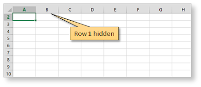
Excel Tip #030 Row 1 Is Missing. How to unhide? As you know, hiding and unhiding rows in Excel is simple as selecting them, right-clicking and choosing Hide or Unhide . The trick to selecting hidden rows, is to select a row above or below and then drag to included the hidden rows. For example, if you accidentally hide row 1 of your worksheet or inherit someone else's worksheet with one or more of the top rows hidden, you may be wondering how to unhide them since apparently you cannot select them. Row 1 Hidden There is a really easy solution. 1) Point to the row 2 header , press the left mouse button and drag upward to the top of the worksheet. Although you cannot see it, row 2 and row 1 are now selected 2) Right click anywhere on row 2 3) Choose Unhide from the right-click menu Unhiding hidden Row 1 NOTE : This also works for multiple hidden rows. There is another method of doing the same if Row 1 is hidden. 1) Go to the top left corner of the sheet abov

Subtotal Dates By Month (or) Year

Image
Excel Tip #029 Subtotal Dates By Month (or) Year There may be times when you want to subtotal your data by month and year, however simply Subtotaling a column of dates won't work because that will create a subtotal for each day. Subtotal Dates - Example Here's a trick you can use to create subtotals for each month while ignoring the day... 1) Sorted your dates by selecting a single date within the table and from the Data tab click the sort A>Z button; 2) Next you need to apply a date/number format that displays the month but not the day (e.g. mmm yyyy). To do this, from the Number group on the Home tab, click the Number Format dropdown (or press CTRL+1) and choose More Number Formats ..., then click Custom and enter mmm yyyy in the Type box. All of the dates now display the month and year (e.g. Apr 2015) Formatting Dates 3) To subtotal your data based on the month and year in the Date column, from the Data tab, click Subtotal,. in the Subtotal dial

Use of Function keys in Excel

Image
Excel Tip #028 Use of Function keys in Excel Most of us know few function keys that are used as shortcuts in Excel, but hardly make use of it. Either because of the keyboard settings or due to the scarcity of the knowledge. Below, the use of function keys are tabulated along with their combinations which will make your life much more easier. Function Key = F1 to F8 Function Key = F9 to F12 Try to use these Function key shortcuts in your day to day tasks and be benefited.

Find And Replace Cell Colors

Excel Tip #027 Find And Replace Cell Colors It is common for Excel users to apply background colors to cells, such as green to indicate for positive, red to indicate warning etc. But how to remove the green fill color from hundreds of cells throughout the workbook without having to do them one by one. Steps to Find cells with a specific Fill color      1) Press CTRL+F to open the Find dialog       2) If you don't see the Format button, click the Options>> button       3) Click the Format... button       4) Click each of the tabs (Number, Alignment, Font, Border, Fill and Protection) and, if the Clear button isn't 'grayed out', click it to clear any formatting from the search criteria       5) Click the Fill tab and choose the color you wish to find     6) Click the Find All button. All of the cells with the Fill color you selected will be listed at the bottom of the Find and Replace dialog To Replace the Fill color in the 'found' cells

Move Columns & Rows Quickly

Image
Excel Tip #026 Move Columns & Rows Quickly I often see Excel users 'moving' a column by inserting a blank column where they want to move the column, drag the original column and drop it in the empty column, the go back and delete the empty original column. Same thing for rows. There is a much, much easier and faster way! Move Columns To move a column (or multiple columns) and insert it (them) between two other columns,       1) Select the column(s) you want to move      2)   Hold down the SHIFT key. Holding down SHIFT tells Excel to 'insert' the columns      3)   Point to the edge of the selected column(s)      4)   Press and hold your left mouse button to drag and position the 'insertion bar' where you want to move the column(s)      5)   Release the mouse button, then release the SHIFT key Move Columns Alternatively,  Right-click column heading you want to move, select Cut, right-click the column heading to the right of where yo

Return the last value in a list

Image
Excel Tip #025 Return the last value in a list You would have faced some situations where you want to get the last value in the list. And this list will not be static, the list will grow further and still the the last value has to be returned . Quite interesting...! There might be multiple ways but as far I know, there are 2 ways in which we can get this done. But as far I consider, there are loopholes in all the 2 methods . Let us get in detail with all the 2 methods. Method 1 This method uses the function LOOKUP . Let us see get to know about this function. LOOKUP function returns a value from a range (one row or one column) or from an array. The syntax is: LOOKUP( lookup_value, lookup_range, [result_range] ) (or) LOOKUP( lookup_value, lookup_range ) We are going to use a hidden excel function in this method which is 9e9 . So what does this 9e9 give?  9e9 is just a notation for 9,000,000,000 which is considered as the largest value in the array . I

Calculate Weighted Average

Image
Excel Tip #024 Calculate Weighted Average Excel makes it extremely easy to calculate the average of data by using the AVERAGE function. But what if some of the values have more "weight" than others? For those cases, you'll need to calculate the Weighted Average . Although Excel doesn't have a weighted average function, it does have a function that does most of the work for you: SUMPRODUCT . In order to calculate the weighted average, we are having 2 columns of data. The first column contains the grades for each assignment and the second column contains the weights. A higher weight will cause the data (assignment) to have a greater effect on the final grade. The weights can also be greater than 100% but it would be meaningful if it is 100% Below is the example data containing 5 assignments along with their marks and the weights. Example - Weighted Average Before going to the example, let us learn about SUMPRODUCT. This function multiplies the correspo